3.1.1 Use of SI units and their prefixes

Content

Fundamental (base) units.
Use of mass, length, time, amount of substance, temperature, electric current and their associated SI units.
SI units derived.
Knowledge and use of the SI prefixes, values and standard form.
The fundamental unit of light intensity, the candela, is excluded.
Students are not expected to recall definitions of the fundamental quantities.
Dimensional analysis is not required.
Students should be able to use the prefixes: T, G, M, k, c, m, μ, n, p, f.
Students should be able to convert between different units of the same quantity, e.g. J and eV, J and kWh.

The fundamental base units are as follows:

The Ampere (A) for electrical current, the candela (cd) for luminous intensity, the Kelvin (K) for thermodynamic temperature, the kilogram (kg) for mass, the metre (m) for length, the mole (mol) for amount of a substance, the second (s) for time.

Examples of deriving SI units from other units are:

Joule = kg.m².s^-2, watt= kg.m².s^-3. These units can be derived from equations i.e. From the equation P=Fv, where the unit of power is the newton. F=ma so f=kg.m.s^-2, so kg.m.s^-2 multiplied by ms^-1 (which is the “v” from p=fv) equals kg.m².s^-3. So these are the derives S.I units of power which has the unit of the watt.

SI Prefixes, values and standard form.

Above is a table of the SI prefixes and values, with their respective symbols. The symbols can be used in place of using standard form, however sometimes you will be required to use standard form, which can be done as follows…

Converting between J and eV, J and kWh.

3.1.2 Limitation of physical measurements

Content

Random and systematic errors.
Precision, repeatability, reproducibility, resolution and accuracy.
Uncertainty:
Absolute, fractional and percentage uncertainties represent uncertainty in the final answer for a quantity.
Combination of absolute and percentage uncertainties.
Determine the uncertainties in the gradient and intercept of a straight-line graph.
Individual points on the graph may or may not have associated error bars.
Students should be able to identify random and systematic errors and suggest ways to reduce or remove them.
Students should understand the link between the number of significant figures in the value of a quantity and its associated uncertainty.
Students should be able to combine uncertainties in cases where the measurements that give rise to the uncertainties are added, subtracted, multiplied, divided, or raised to powers. Combinations involving trigonometric or logarithmic functions will not be required.
Random and systematic errors.
A random error is one which is always present in data, and is due to readings that vary randomly, with no recognizable trend or bias. A random error could be caused by a faulty instrument, human error or a poor technique.
A systematic error is one which follows a pattern/trend, or a bias, and results in readings that systematically differ from the true mean reading. Systematic errors could be caused by a non-zero reading at the beginning i.e. on a voltmeter/ammeter. There could also be a consistent error in a technique used, or a calibration error in the instrument.
Precision, repeatability, reproducibility, resolution and accuracy.
Precision can be either precision of an instrument, or precision of a measurement. Precision of an instrument is the smallest non-zero value that can be measured, also referred to as the resolution of that instrument. The precision of a measurement is the degree of exactness of a measurement, usually referred to as the uncertainty of the readings used to obtain a measurement.
Uncertainty
This is the precision of a measurement due to the instrument used.
Absolute, fractional and percentage uncertainties represent uncertainty in the final answer for a quantity.
The absolute uncertainty is the size of the range of values that the ‘true’ value lies. For example in a measurement of 10.0m, the uncertainty is ±0.1m. So the absolute uncertainty would be 10.0m ± 0.1m, as this is the range of values that could be the ‘true’ value.
Fractional uncertainty is simply the calculating by dividing the uncertainty by the value of the data. For example: 1.2 s ± 0.1s, the fractional uncertainty would be equal to 0.1 / 1.2 = 0.08.
Percentage uncertainty is just the fractional uncertainty multiplied by 100. So for the fractional uncertainty given above, the percentage uncertainty would be 8.0%. So this tells us that the value of 1.2 can deviate by ± 8%.
Combination of absolute and percentage uncertainties.
1. If you add or subtract the two (or more) values to get a final value
The absolute uncertainty in the final value is the sum of the uncertainties. For example:
10.0 ± 0.1 mm + 4.0 ± 0.1 mm = 14.0 ± 0.2 mm
10.0 ± 0.1 mm – 4.0 ± 0.1 mm = 6.0 ± 0.2 mm
1. If you multiply one value with absolute uncertainty by a constant the absolute uncertainty is also multiplied by the same constant. For example:
2 x (10.0 ± 0.1 mm) = 20.0 ± 0.2 mm
1. If you multiply or divide two (or more) values, each with an uncertainty you add the % uncertainties in the two values to get the % uncertainty in the final value. For example:
10.0 ± 0.1 mm x 4.0 ± 0.1 mm
This is
10.0 ± 1% x 4.0 ± 2.5%
So the final result is
40.0 ± 3.5%
1. If you square a value, then you multiply the % uncertainty by 2. If you cube a value, then you multiply the % uncertainty by 3. If you need the square root of a value, you divide the % uncertainty by 2.
In the question below, you are told to find the absolute and percentage uncertainty in the value of s when using the equation s = ut + at²/2. This is done by combining the uncertainties of ut, and at²/2.
1. This question applies knowledge of uncertainties from the last topic.
2. First we need to find the percentage uncertainty on ‘ut’. Since ‘ut’ is two values multiplied together, we have to add their percentage uncertainties. This can be done by finding their fractional uncertainty and then multiplying this by 100. For example, for u: 0.1/10.0 = 0.01 which is the fractional uncertainty. We need the percentage uncertainty, which is 0.1 x 100, so 1%. We know that the percentage uncertainty on u is 1%, and on t is 0.5%, so the final percentage uncertainty on ‘ut’ is 200.0 ± 1.5%.
3. On at², we have to find the percentage uncertainty on t, and add it to that of a. ½ does not carry an uncertainty. So we know that the uncertainty on t is 0.5%, so the uncertainty on t² is therefore 0.5% x 2, so 1%. Then we need to find the percentage uncertainty on a, which is 2%, and add this to that of t². This gives an answer of 1000.0 ± 3%.
4. Now we have the percentage uncertainty on the product of ‘ut’ and ‘at²/2’. However these two quantities are added together in the equation s = ut + at²/2, so to add the uncertainties we need to convert to fractional uncertainties.
5. The final answer is therefore 1200 ± 54 as an absolute uncertainty, or 1200 ± 4.5% as a percentage uncertainty. The absolute uncertainty is worked out using either the fractional or percentage uncertainty, as it it just the range of values that the answer could be, using the fractional or percentage uncertainty will give the same answer.
Determine the uncertainties in the gradient and intercept of a straight-line graph
To determine the uncertainty in the gradient of a graph you simply simply add error bars to the first and last point, and then draw a straight line passing through the lowest error bar of the one points and the highest in the other and vice versa. This gives two lines, one with the steepest possible gradient and one with the shallowest, we then calculate the gradient of each line and compare it to the best value. The figure below shows how this is done.

To determine the uncertainty in the y – intercept we do a similar thing as when calculating the uncertainty in gradient. This time however, we check the lowest, highest and best value for the intercept by drawing the different possible intercepts from the different gradients.

Individual points on the graph may or may not have associated error bars.
3.1.3 Estimation of Physical Quantities
Content
- Orders of magnitude.
- Estimation of approximate values of physical quantities.
Opportunities for Skills Development
- Students should be able to estimate approximate values of physical quantities to the nearest order of magnitude.
- Students should be able to use these together with their knowledge of physics to produce further derived estimates also to the nearest order of magnitude.
Orders of Magnitude
An order-of-magnitude estimate of a variable whose precise value is unknown is an estimate rounded to the nearest power of ten. For example, there are two orders of magnitude between 10⁴and 10⁶, so a factor of 10²difference between them.
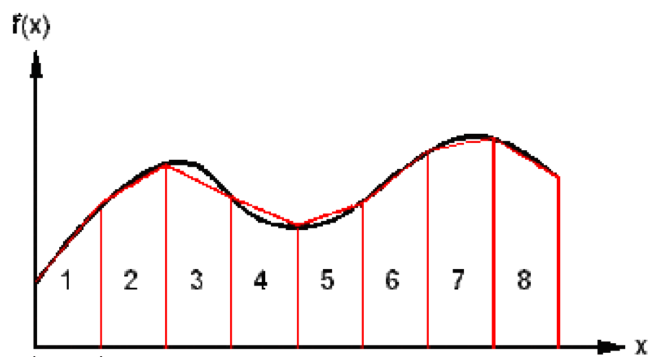
Estimation of approximate values of physical quantities
When making estimates, it is reasonable to give the figure to one or two significant figures since the estimate is not supposed to be completely precise. For example, the mass of a car to be 1000kg, or the length of a football pitch to be 100m. Or you could be asked to estimate the area under a graph of a curved line. This can be done by drawing trapeziums in, so you can calculate the area of regular trapeziums along the line. This is shown in the diagram below:

Sources: